
*UNDER CONSTRUCTION*

Bezier Curve


Note

이 포스트는 고1 금요학술포럼에서의 발표를 글로 옮긴것으로 블로그를 시작하기 전 활동입니다.
발표 당시 PPT는 다음 링크에서 확인 가능합니다.
https://ywbird.github.io/ppt.old/bezier-ppt/[↗]

Vector 이미지

  • Scalable Vector Graphics
  • 확대해도 깨지지 않는 이미지
SVG PNG

왼쪽은 vector 이미지, 오른쪽은 png 이미지.
가능하다면 컴퓨터에서는 Ctrl + +로 확대하거나, 모바일에서 핀치로 확대해서 보면 왼쪽은 픽셀이 보이지 않는 반면, 오른쪽은 픽셀이 보인다.

구현 방식

사실 알고리즘 자체를 구현한것은 Bernstein Polynomial가 먼저였지만, 이를 시각적으로 볼 수 있게 표현한 De Casteljau Algorithm을 먼저 알아보자.

De Casteljau Algorithm

Important

$$ lerp(P_0, P_1, t) = (1-t) \cdot P_0 + t \cdot P_1,\ 0 \leq t \leq 1 $$

$P_0$ 와 $P_1$ 사이의 점 $P$가 존재, $P_0$, $P_1$ 사이 거리 비율로 $P$ 표현
Linear Interpolation - 선형 보간 함수 - lerp

  • 점 2 개 Lerp → Linear Bézier Curve
  • 점 3 개 Lerp → Quadratic Bézier Curve
  • 점 4 개 Lerp → Cubic Bézier Curve
  • 점 N 개 Lerp → $N − 1$ -th Bézier Curve

Linear Bézier

$$ P = lerp(P_0, P_1, t) $$

linear {60%x}

Add

📈 Animated Desmos Graph

Quadratic Bézier

$$ \begin{align} Q_0 &= lerp(P_0, P_1, t) \\ Q_1 &= lerp(P_1, P_2, t) \\ \\ P &= lerp(Q_1, Q_2, t) \end{align} $$

quadratic {60%x}

Add

📈 Animated Desmos Graph

Cubic Bézier
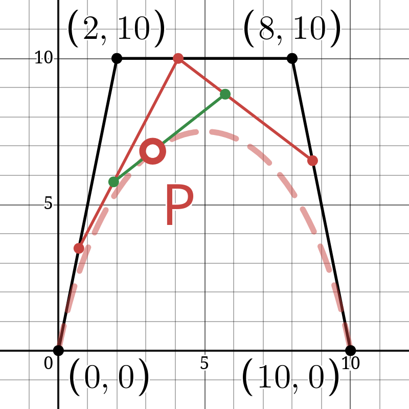
$$ \begin{align} Q_0 &= lerp(P_0, P_1, t) \\ Q_1 &= lerp(P_1, P_2, t) \\ Q_2 &= lerp(P_2, P_3, t) \\ \\ R_0 &= lerp(Q_0, Q_1, t) \\ R_1 &= lerp(Q_1, Q_2, t) \\ \\ P &= lerp(R_0, R_1, t) \end{align} $$

cubic {60%x}

Add

📈 Animated Desmos Graph

이처럼 De Casteljau Algorithm은 $lerp$를 쌓는 방식으로 Bézier Curve를 구현한다.
위에서 구현한 것 이상으로 4차, 5차로도 만들 수 있겠지만, 그 이상의 곡선은 거의 3차 곡선(Cubic Bézier) 여러개를 사용해 거의 똑같이 만드는것이 가능함에 더해 계산 효율성마저 떨어지기 때문에 잘 사용하지 않는다.

Bernstein Polynomial

조절점 $P_0, P_1, P_2, ..., P_n$ 에 대한 Bézier Curve


$$ P(t) = \sum_{i=0}^n P_i {n \choose i}(1-t)^{n-i}t^i P_i,\,0 \leq t \leq 1 $$

n=3 일때

$$ \begin{align} P(t) &= \sum_{i=0}^n {n \choose i}(1-t)^{n-i}t^i P_i \\ &= (1-t)^3 \cdot {\color{red}P_0} + 3 \cdot (1-t)^2 \cdot t \cdot {\color{green}P_1} + 3 \cdot (1-t) \cdot t^2 \cdot {\color{teal}P_2} + t^3 \cdot {\color{orange}P_3} \end{align} $$
$$ \begin{align} y&={\color{red}(1-t)^3}\\ y&={\color{green}3 \cdot (1-t)^2 \cdot t}\\ y&={\color{teal}3 \cdot (1-t) \cdot t^2}\\ y&={\color{orange}t^3}\\ \end{align} $$

bern {60%x}

Add

📈 Animated Desmos Graph

계산해보면, 위 항들의 합은 항상 $1$임을 알 수 있는데, 각 점에 가중치를 준다고 생각하면 편할 듯 하다.

관계?

De Casteljau Algorithm에서 3차 곡선의 식을 정리하면 아래의 식으로 Bernstein Polynomial에서 $n=3$일때의 식과 완전히 동일하다.

$$ \begin{align} P(t) &= \sum_{i=0}^n {n \choose i}(1-t)^{n-i}t^i P_i \\ &= (1-t)^3 \cdot {\color{red}P_0} + 3 \cdot (1-t)^2 \cdot t \cdot {\color{green}P_1} + 3 \cdot (1-t) \cdot t^2 \cdot {\color{teal}P_2} + t^3 \cdot {\color{orange}P_3} \end{align} $$

Webmentions(?)

Q. Why isn't my webmention not appearing?

A. I deploy this site not so often and this site is static site. So don't expect your webmention to appear instantly. Thanks for the webmention and sorry for the inconvenience.
last deployed: see footer