Important
This post assumes familiarity with Lambda Calculus .
Having been interested in lambda calculus and having previously explored Lambda Diagram , I became interested in visualizing lambda calculus.
While watching the video below, I wondered whether lambda calculus could be visualized as a two-dimensional mosaic.
Lambda Treemap
Lambda calculus has three syntactic forms.
- Variable
- Abstraction
- Application
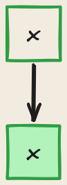
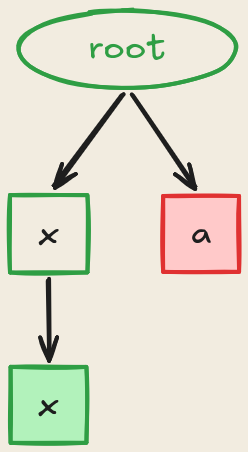
Each form can be represented in a binary tree.
- Each variable, abstraction, and application is a node.
- A variable is a leaf node.
- An abstraction is a node marked to indicate that it is an abstraction.
- In an application, the lhs is the function being applied and the rhs is the argument.
| $x$ | $\lambda x . x$ | $(\lambda x.x)\,a$ |
|---|---|---|
 |  |  |
| $3$ = $\lambda f\,x. f(f(f\,x))$ |
|---|
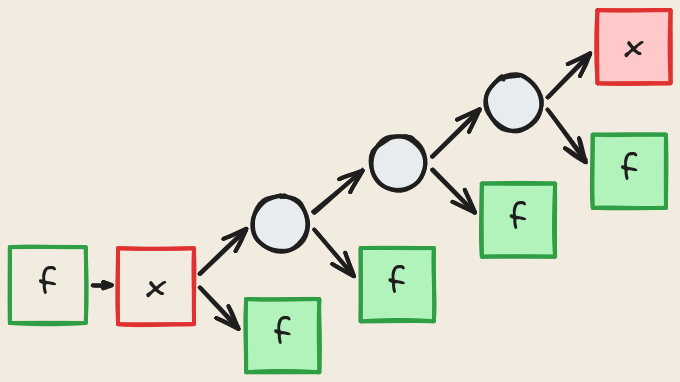 |
A binary treemap is another way to represent a binary tree, so it can likewise be used to visualize lambda calculus.
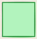
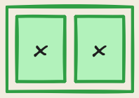
First, a variable is represented by a simple colored rectangle.
$x$
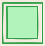
Second, an abstraction is represented by a colored border surrounding the lambda term.
$\lambda x.x$
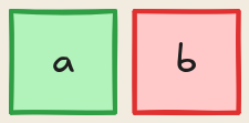
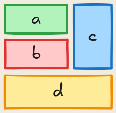
Third, an application is represented as a binary treemap whose nodes are lambda terms.
$(a\,b)$
$(a\,b\,c\,d)$
$\lambda x. x\,x$
Church Numeral
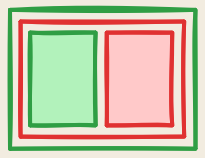
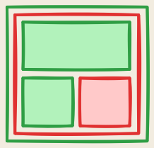
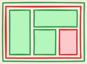
Next, Church numerals can be represented as follows.
| $1 = \lambda f\,x. f\,x$ | $2 = \lambda f\,x.f( f\,x)$ | $3 = \lambda f\,x. f(f(f\,x))$ |
|---|---|---|
 |  |  |
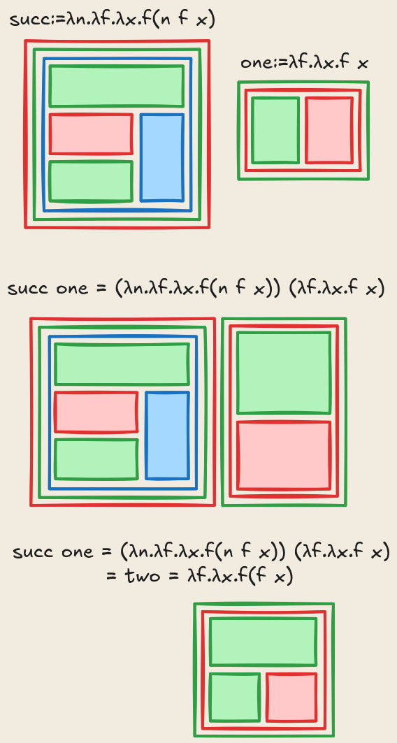
Beta Reduction
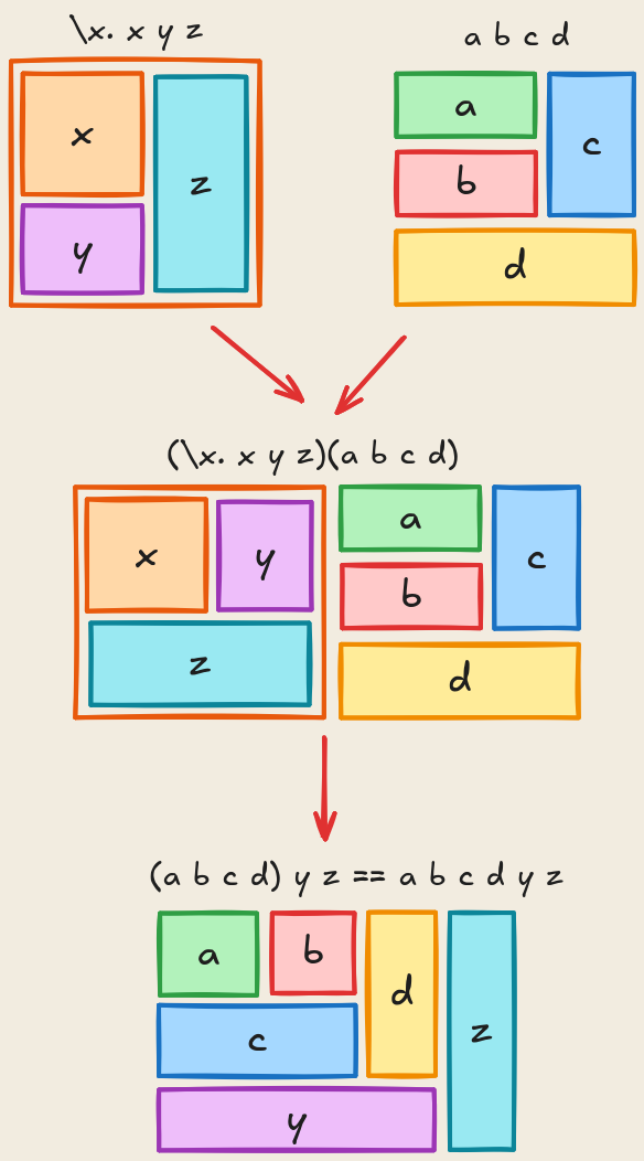
To perform an application, replace every rectangle (variable) corresponding to the abstraction’s border color with the argument treemap.
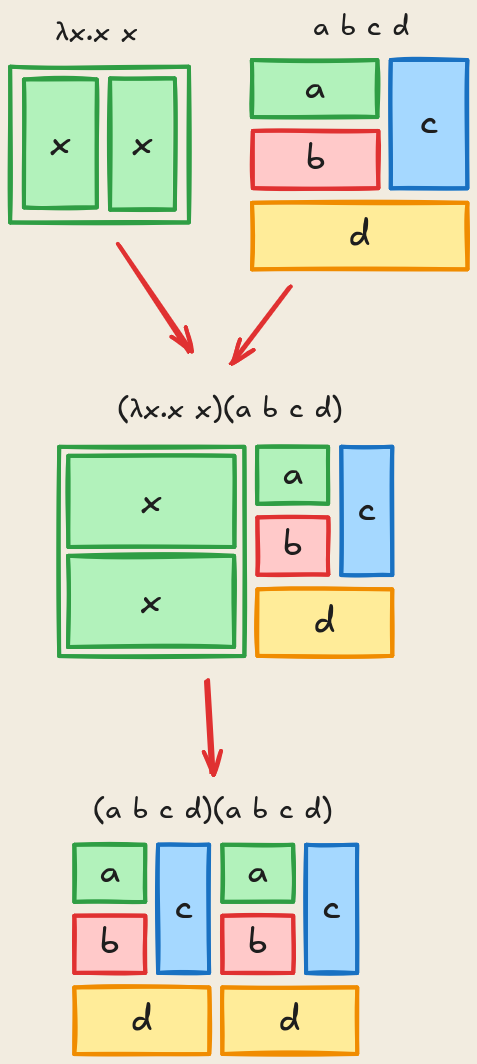
During application, the expression’s orientation may change, swapping its vertical and horizontal orientations.
Try It Yourself
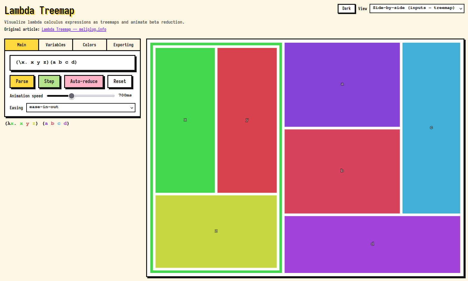
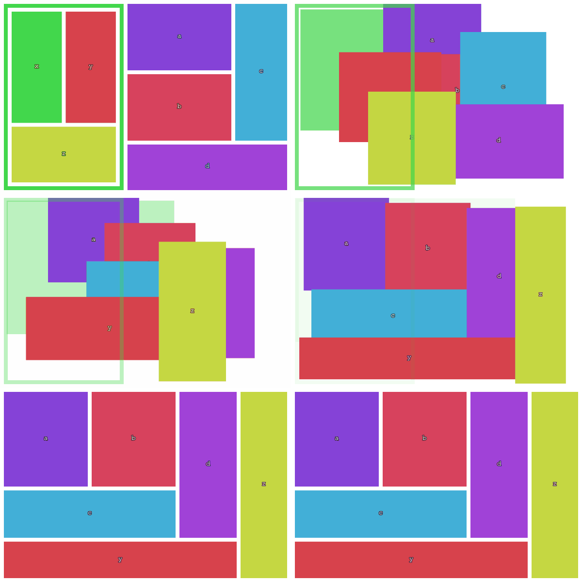
I implemented automatic generation and animation of lambda treemaps through vibe coding.
https://ywbird.github.io/slop-lambda-treemap/[↗]
Appendix
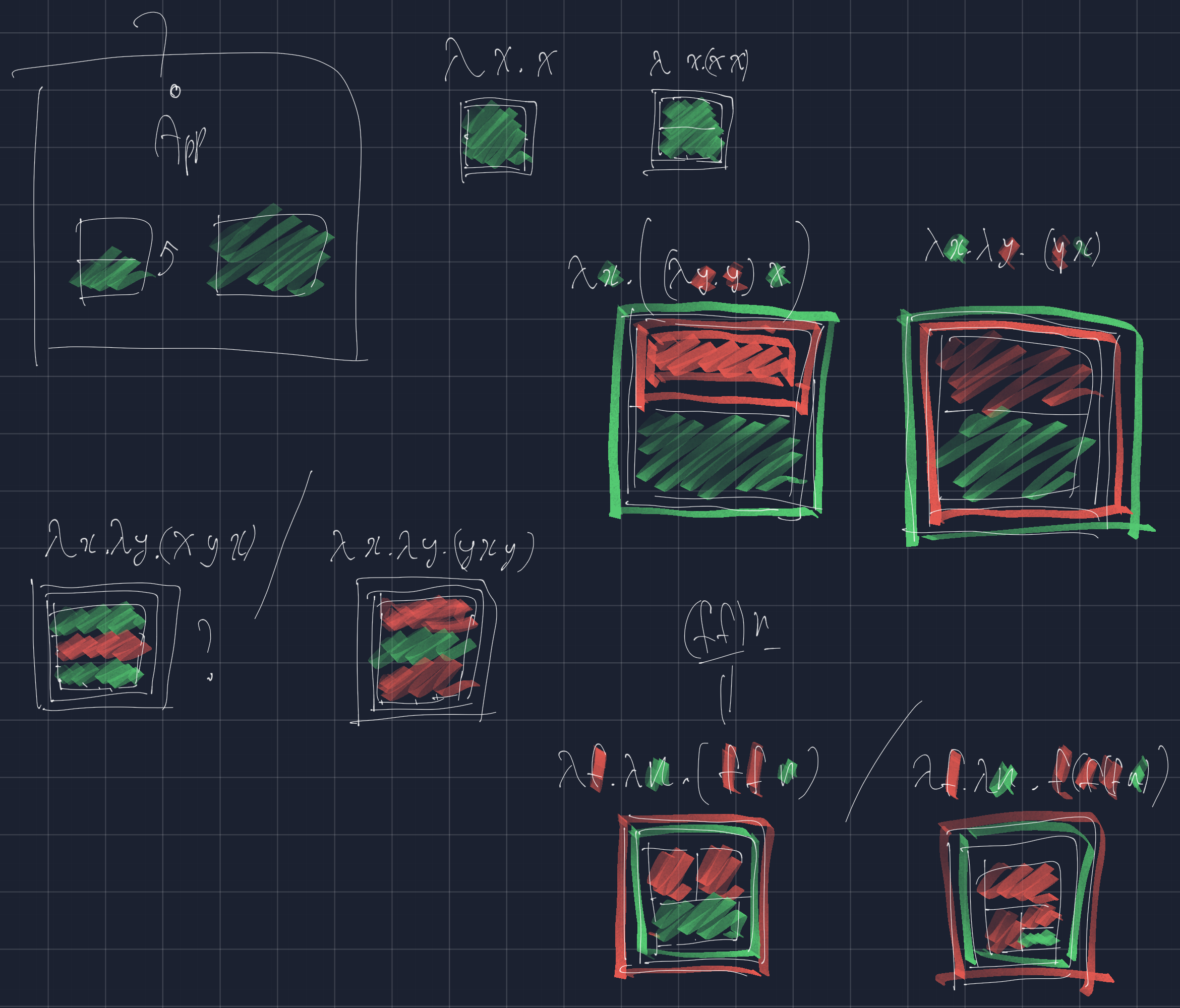
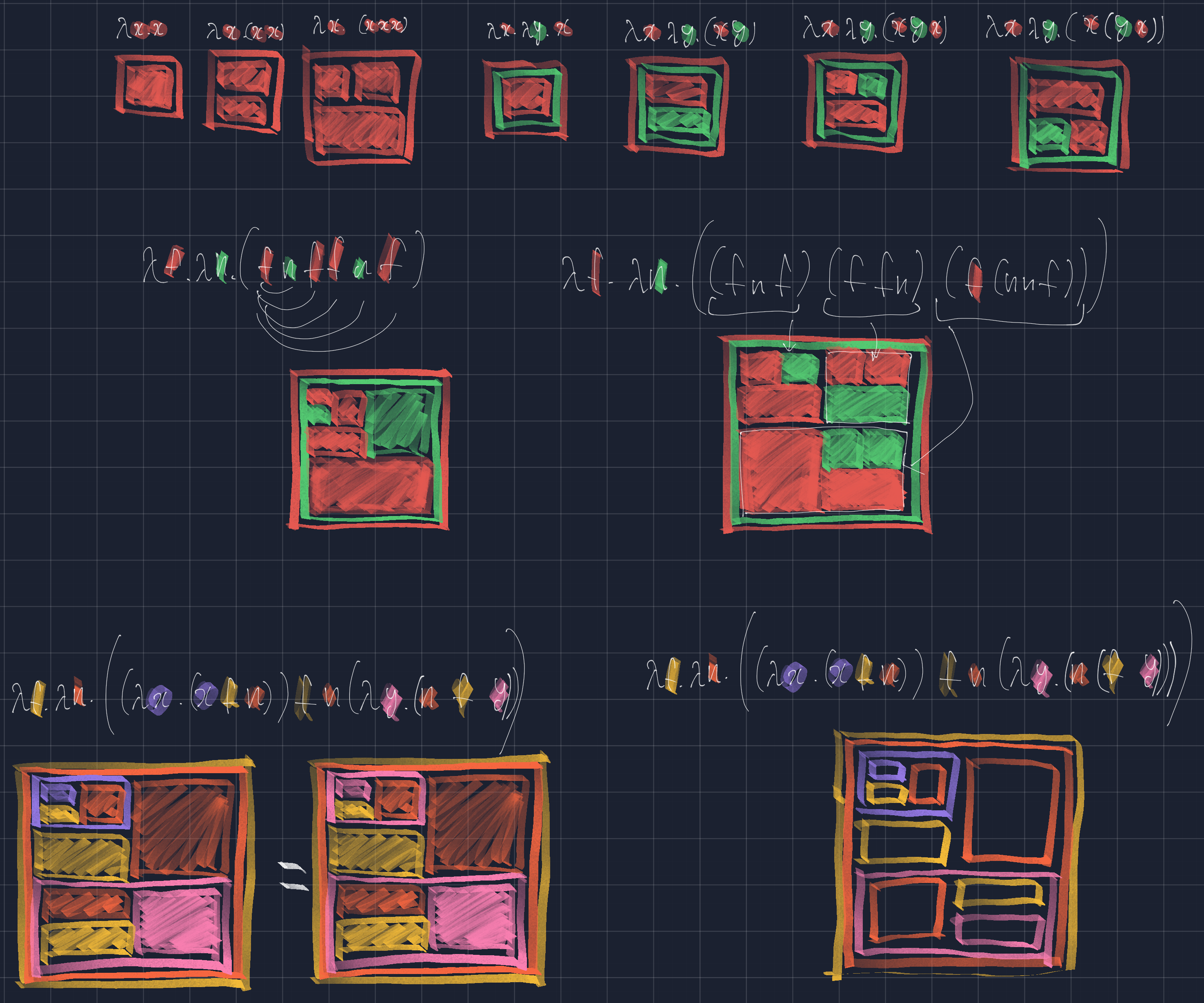
Appendix A: Production Sketches
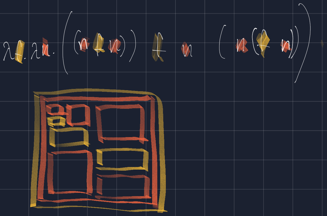
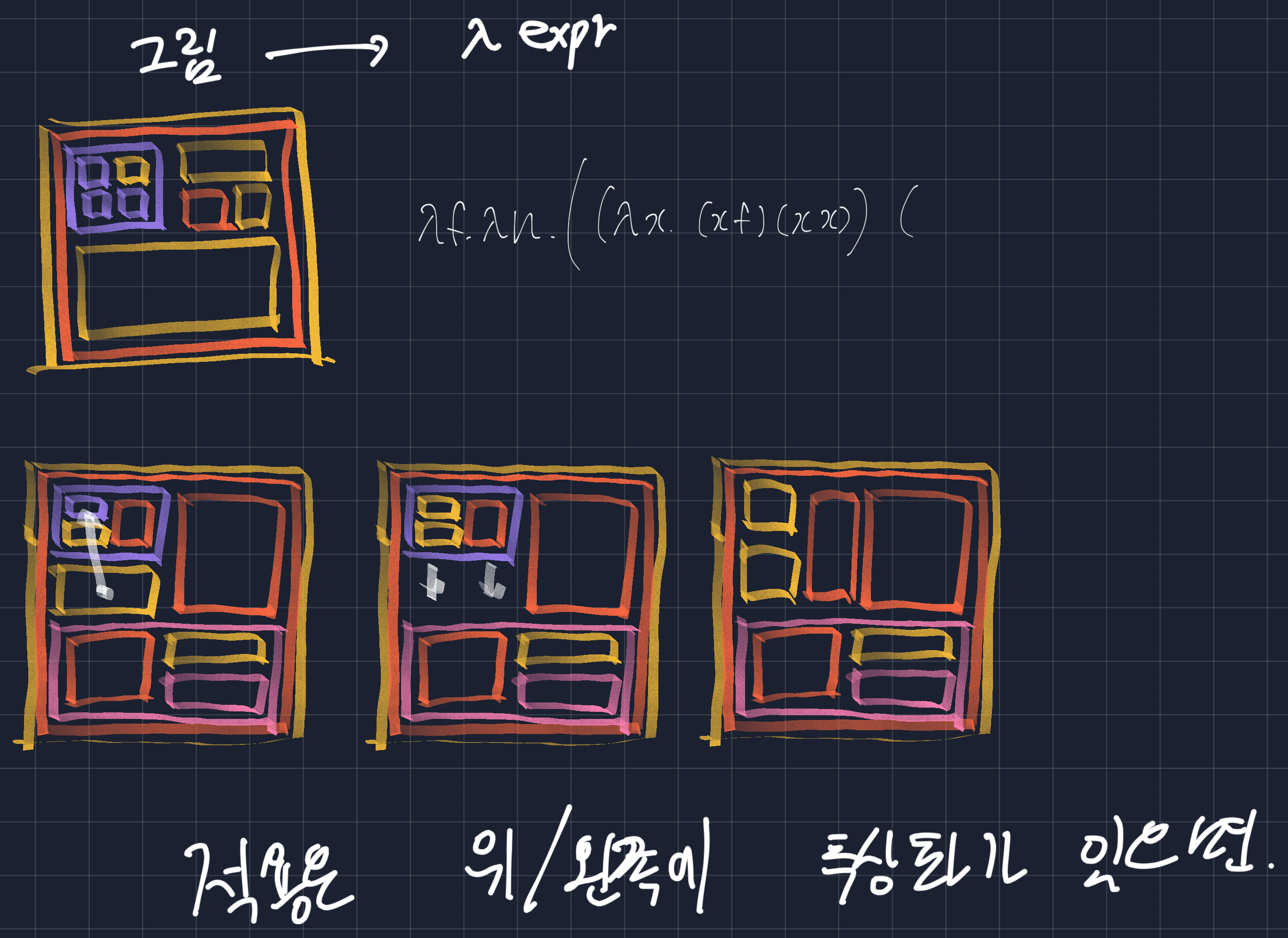
Appendix B: Design Process
In Lambda Diagram, each variable is drawn as a vertical line, an application as a horizontal line, and an abstraction (variable declaration) as a horizontal line at the top.

However, in a rectangle-based visualization, rectangles inevitably become progressively smaller. I thought connections such as lines extending from abstractions (variable declarations), as in Lambda Diagram, would become ambiguous and confusing. So for this project, I defined each variable by a color and indicated it with a border around the rectangle.
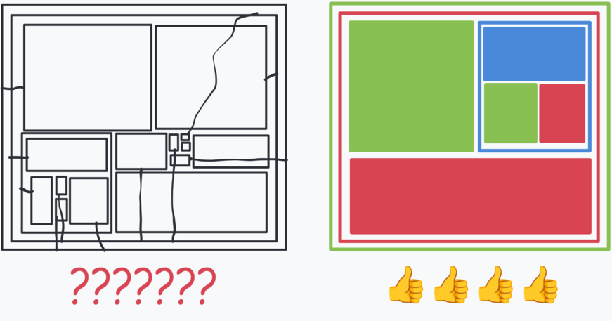
At first, I planned to arrange each application alternately horizontally and vertically around a single block, as shown below.
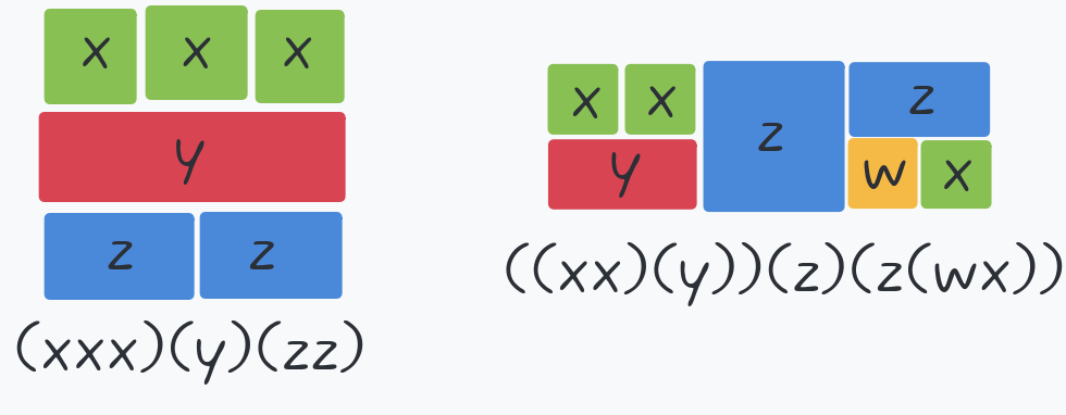
However, the problem was that several expressions could generate mosaics of the same form.
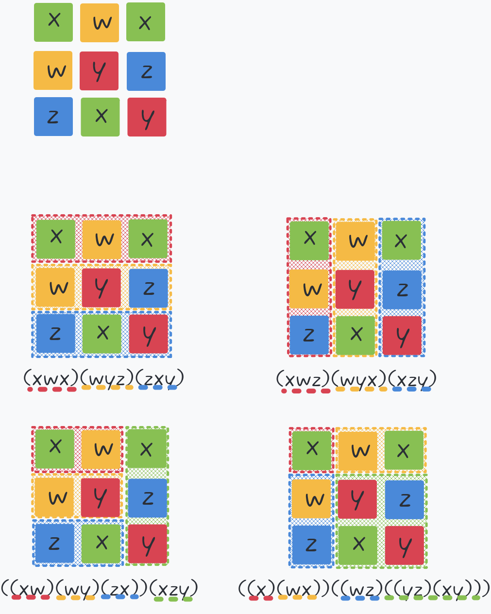
Conversely, a single expression could generate mosaics in several different forms.
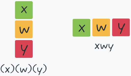
So I decided to draw every application by alternating between horizontal and vertical layouts.
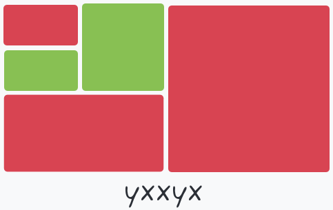
While looking into ways to partition rectangles at this point, I discovered that what I had been naturally making all along was a binary treemap.
Appendix C: Further Analysis of Lambda Diagram
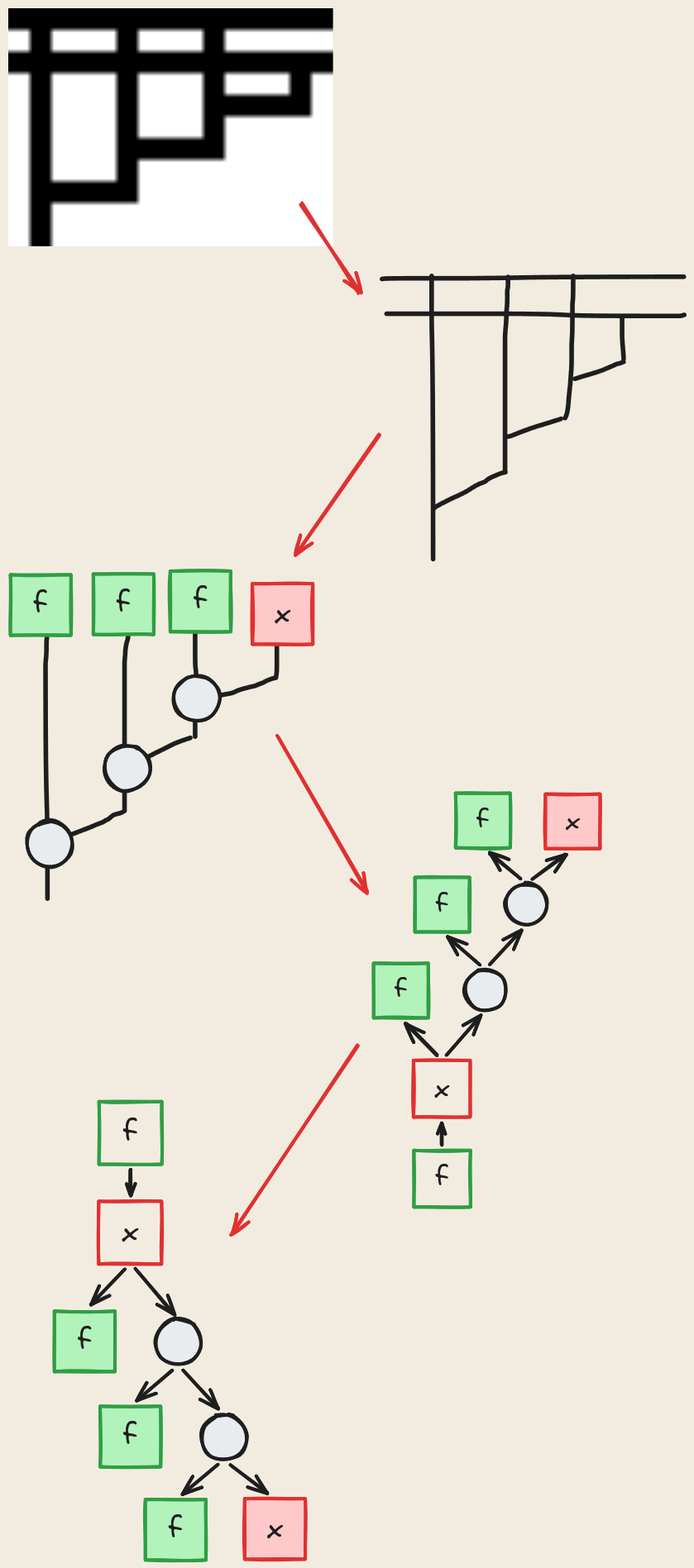
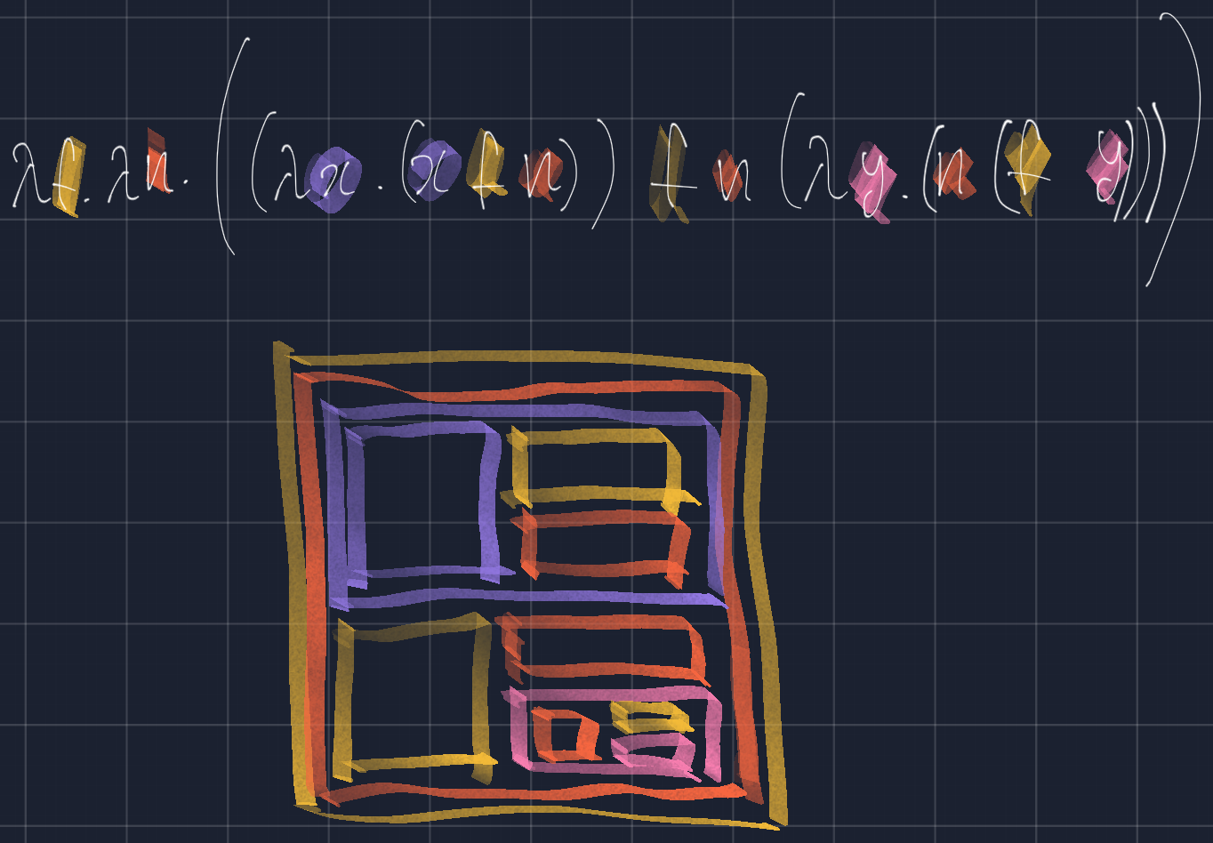
tromp’s Lambda Diagram[↗] is, in fact, a binary tree.
For example, consider Church numeral 3.